We organized the Workshop on Symbolic Regression and Equation Discovery as a subevent within WCCI/CEC 2026 in Maastricht, Netherlands this year. After several years of hosting it at GECCO, it was a great opportunity for meeting new people, discussing SR developments, and sharing ideas.

For the first time, we used OpenReview as a platform to organize paper submissions and reviews. We received 8 submissions and accepted 5 papers, which were presented during the workshop. The accepted papers and review discussions are archived on OpenReview.

Workshop Overview

Program

Two invited talks and four contributed talks were presented during the workshop.

• Invited Talk: "Exhaustive Symbolic Regression: Learning Physics directly from Data", Harry Desmond
• "Learning Parametric Nitrogen Fertilizer Response Curves Using Neuro Symbolic Regression", Giorgio Morales, John Sheppard
• "SRToolkit: Shared Infrastructure for Symbolic Regression Research", Sebastian Mežnar, Ljupco Todorovski, Sašo Džeroski
• Invited Talk: "Evolution of mutation + Genetic and agentic symbolic regression of distributed rate-and-state friction models", Marco Virgolin
• "Prediction Intervals and Confidence Regions for Symbolic Regression Models based on Likelihood Profiles", Fabricio Olivetti de Franca, Gabriel Kronberger
• "Generalized Residuals Symbolic Regression", Rory Sweeney, Takfarinas Saber, James McDermott

Harry Desmond presented exhaustive symbolic regression and in particular their formulation for the calculation of total description length of symbolic regression models, combining model accuracy and complexity for ranking expressions. He then presented several applications and their results in astrophysics including modeling of universe expansion and the radial acceleration relation of galaxies.

Marco Virgolin gave a nice overview of different approaches to mutation in the history of symbolic regression, from initial "tree twiddling" operators to agentic LLM-based approaches. He discussed them within a unified framework of expression variation operators in different algorithms. A short demo in the end showed how agentic-AI based on LLMs can be useful for finding equations in settings where a single evaluation is expensive, such as in physics simulations.

The main takeaway from Marco's talk is that if fitness evaluation is costly, it is worth to use more informed mutation operators to guide the search, while for cheap fitness evaluation, simple mutation operators are sufficient. Make sure to check out his automodel skill. Application to tyre friction modelling: https://github.com/Unlayer-AI/friction-modeling-symreg2026

Discussion

The workshop concluded with a discussion session on relevant future research directions for symbolic regression.

The discussion revolved around integration of prior knowledge into symbolic regression. Some partial solutions which are often application-specific have been proposed e.g. for limit behavior, symmetries, structural preferences [1, 2, 3]. However, it is unclear how those can be expressed, generally to allow SR search processes to consider diverse background knowledge. In a Bayesian formulation we could potentially express this using priors. There are also other possibilities, such as integrated directly into ML loss functions or as secondary objectives. A study was mentioned where neural networks were used in an interactive learning scenario to learn human preferences using interactive feedback from pairwise comparisons. LLMs may provide another avenue for understanding and reacting to background knowledge in written form. The potential of using fuzzy computing ideas for handling human preferences was also mentioned.

Another topic that was raised is that SR community could benefit from research directed into describing SR algorithm behavior. A lot of comparison of methods is based on the results only, i.e. whether method A beats method B in performance. Currently, there is a lot of momentum in the development of different SR methods also in related AI-focussed domains, but there is no clear understanding of the (dis)similarities of methods. How can all of this busyness be directed to develop something substantially new, to prevent that we are re-inventing / discussing the same things over and over again? Visualizations of algorithm internals, such as inheritance patterns, diversity, or inheritability of solution properties could be especially insightful to get a better understanding of algorithm behavior.

Handling uncertainty in SR was a topic in multiple presentations: in the form of uncertainty-aware model selection (based on DL, or Bayesian information criterion) which automatically prefers less complex models when data is scarce or noisy, and for calculating parameter confidence intervals and prediction intervals for symbolic regression models.

Prior work looking into using symbolic regression with vectorial input values was briefly discussed as well [4, 5, 6, 7].

Plans for 2027

We are still undecided where to host the next workshop in 2027. We are considering both GECCO and CEC, and we will announce the location and dates on the workshop website once decided.

We are also interested in hosting a symbolic regression / equation discovery workshop at one of the large AI conferences (NeurIPS, ICML, ICLR, AAAI, IJCAI) in 2027. If you are interested in co-organizing such a workshop, please contact us.

Additionally, we try to host a small, in-depth, invitation-only multi-day SymReg event most likely in the EU in 2027. Let us know if you are interested in participating in such an event.

Finally, I want to thank my co-organizers: Fabricio Olivetti, William LaCava and Steven Gustafson as well as the members of the Programme Committee (Deaglan J. Bartlett, Geoffrey F. Bomarito, Harry Desmond, Alcides Fonseca, Johannes Koch, Alessandro Lucantonio, James McDermott, Julia Reuter, Colm O'Riordan, Giovanni Squillero, Alberto Tonda, Leonardo Trujillo, Bernhard Werth, Stephan Winkler, Aisha Yousuf) for their help in reviewing the submitted papers.

In the last post we introduced the idea of e-graphs and how it can play an important role with equation discovery (aka symbolic regression). We also introduced eggp [1], the first equation discovery algorithm that takes advantage of e-graphs by using it as a powerful database system and enforce novelty.

We also briefly introduced r🥚ression [2], a Python tool that allows us to explore the power of e-graphs in different scenario. In this post, we will play a bit more with this tool to show how powerful e-graphs can be as a go to tool for equation discovery.

For a gentle introduction to e-graphs and equality saturation, see the previous part of this blog post.

First things first

For this experiment, we will use a dataset generated from the function below (inspired by the Salustowicz function [3] [10]):

$$ e^{-x/1.2}, x^3 \left(\cos(x), \sin(x)^2 - 3.1415\right) $$

Let's generate data points in the range $[0, 10]$ while adding a bit of Gaussian noise:

x = np.arange(0, 10, 0.05)
y = np.exp(-x/1.2)*x**3*(np.cos(x) \
    * np.sin(x)**2 - 3.1415) \
    + np.random.normal(0, 0.05, x.shape)

To make things a bit more interesting for this post, we will use just the middle part for training and the rest as a test set:

lb, ub = 2.1, 5
x_sel = x[(x>lb) & (x<ub)].reshape(-1,1)
y_sel = y[(x>lb) & (x<ub)]
x_ood = x[(x<=lb) | (x>=ub)].reshape(-1, 1)
y_ood = y[(x<=lb) | (x>=ub)]

Plotting the training set as red dots and the test set as green dots, we have:

We are, of course, making things harder for symbolic regression:

1. The relationship is nonlinear.
2. The training set is insufficient to guarantee an unique global optima.

In any case, the purpose here is to show how we can use r🥚ression to explore alternative models.

Laying the egg 🥚

We can create an initial e-graph for this dataset using eggp. As mentioned in the previous post, this algorithm uses e-graphs to enforce the generation of new expressions, avoiding redundancy in the search.

from eggp import EGGP
import pandas as pd

reg = EGGP(gen=200, nPop=200, maxSize=25, \
      nonterminals="add,sub,mul,div,log,power,sin,cos,abs,sqrt", \
      simplify=True, optRepeat=2, optIter=20, folds=2,  \
      dumpTo="vlad.egg")
reg.fit(x_sel, y_sel)

Some observations:

• The non-terminal set is large in order to generate many different alternative models.
• We are not running for a large number of iterations, so we could possibly find better models with proper settings.
• The maximum size is larger than the true equation.

We are saving the final e-graph into the file named vlad.egg so we can explore it after the search. Looking at the results we can see the Pareto front with different trade-offs of accuracy and size.

Hatching the egg 🐣

Now, let's load the e-graph into r🥚ression:

from reggression import Reggression
egg = Reggression(dataset="vlad.csv", loadFrom="vlad.egg")

If we look at the top-5 models, we can see small variations of the top performing with similar fitness (negative MSE) values.

egg.top(5)[["Latex", "Fitness", "Size"]]

Some of these functions behave similarly while others display a different behavior when looking outside of the training region:

We can also plot the best models while limiting the maximum size:

model_top(egg.top(n=10, filters=["size <= 10"]), n, x, y)

We can see even more different behaviors compared to the previous plot but, sill, none of them are even close to the correct one :-(

Since we are still far from the true expression, let us investigate the distribution of the tokens of the top 1000 generated expressions.

egg.distributionOfTokens(top=1000)

This command returns a table with the number of times each token was used in the top expressions and the average fitness of the expressions that contains such token. The table is ordered by average fitness (negative MSE).

Apart from the first rows that displays the terminals, we can see that the absolute value function is frequently used and often contributes to a lower fitness, even though it is not present in the ground-truth expression.

When we have partial functions such as log and sqrt, the absolute value can help "fixing" invalid inputs.

Sine and cosine are ranked next, but with cosine being more often used. The exponential is rarely used and particularly with a worse average fitness than the other tokens. The reason for this could be that fitting parameters inside an exponential function can be tricky depending on the initial values.

We can verify that by plotting the top 5 expressions with the pattern $e^{\square_0}\square_1$ with the command:

egg.top(n=n, pattern="exp(v0)*v1")

as we can see, still not a very good fit, as expected.

With a little help from my friends 🐣🐤

We can try our luck with another SR method, such as Operon [4], and insert the obtained expressions into the e-graph:

from pyoperon.sklearn import SymbolicRegressor
regOp = SymbolicRegressor(objectives=['mse','length'], max_length=20, allowed_symbols='add,sub,mul,div,square,sin,cos,exp,log,sqrt,abs,constant,variable')
regOp.fit(x_sel, y_sel)
f = open("equations.operon", "w")
for eq in regOp.pareto_front_:
  eqstr = regOp.get_model_string(eq['tree'])
  fitness = -eq['mean_squared_error']
  print(f"{eqstr},{fitness},{fitness}", file=f)
f.close()
egg.importFromCSV("equations.operon")

Plotting the top-5 expressions we get:

Still no luck! But we didn't make things easy for SR anyway!

We can insert the ground-truth expression to see whether the parameter optimization is capable of converging to the true parameters and if the fitness is better than what we have.

egg.insert("exp(x0/t0)*(x0^3)*(cos(x0)*(sin(x0)^2)-t1)")

The answer is YES! We can get the ground-truth expression with enough iterations and a larger amount of luck :-) Or, we can even resort to adding some constraints [5]...

It's all the same, no matter where you are 🐥🐥🐥

We can also use r🥚ression to check whether two or more expressions are equivalent. Let's say we want to see whether $(x+3)^2 - 9$ and $x(x + 6)$ are the same.

First, we create an empty e-graph:

newegg = Reggression(dataset="vlad.csv", loss="MSE")

Next, we add both expressions while storing their e-class ids:

eid1 = egg.insert("(x0 + 3)**2 - 9").Id.values[0]
eid2 = egg.insert("x0*(x0 + 6)").Id.values[0]
print(eid1, eid2)
> 6, 9

Initially, their ids are going to be different, since until now they are distinct to each other as far as the e-graph is concerned.

Now, the main idea is that we run equality saturation to produce all the equivalent forms of each one of these expressions following a set of rules, such as:

$$ (x + y)^2 \rightarrow x^2 + y^2 + 2xy $$

If the set of rules are sufficient to produce at least one common expression departing from the first and from the second expressions, they will eventually be merged, and their e-class id will become the same.

We can run some iterations of equality saturation using the command:

egg.eqsat(5)

And, now, their ids should be the same!

print("Id of the first equation: \n", egg.report(eid1).loc[0:1, ["Info", "Training"]])
print("Id of the second equation: \n", egg.report(eid2).loc[0:1, ["Info", "Training"]])
> Id of the first equation: 16
> Id of the second equation: 16

After running equality saturation, we can also retrieve a sample of the equivalent expressions for that e-class id:

egg.getNExpressions(eid1, 10)

Leading to:

$$ ((6.0 + x) * x) \\ ((x + 6.0) * x) \\ ((x * 6.0) + (x ^ 2)) \\ ((x * 6.0) + (x ^ 2)) \\ (0.0 + ((6.0 + x) * x)) \\ (0.0 + ((x + 6.0) * x)) \\ ((2.0 * (x * 3.0)) + (x ^ 2)) \\ ((2.0 * (3.0 * x)) + (x ^ 2)) \\ (((x * 3.0) * 2.0) + (x ^ 2)) \\ (((3.0 * x) * 2.0) + (x ^ 2)) \\ $$

This can potentially be used to integrate e-graphs with other genetic programming algorithms or even reward based algorithms such as Monte Carlo Tree Search [6] [7] and Deep Reinforcement Learning [8], and LLMs [9].

Stay tuned!

As we can see, there is still a vast ground to be explored with the combination of e-graphs and symbolic regression! Stay tuned for our next exciting work on this topic.

Try it yourself

The full Jupyter Notebook is available here and the rEGGression repository also host some tutorials

References

[1] de França, Fabrício Olivetti, and Gabriel Kronberger. "Improving Genetic Programming for Symbolic Regression with Equality Graphs." Proceedings of the Genetic and Evolutionary Computation Conference. 2025.

[2] de França, Fabrício Olivetti, and Gabriel Kronberger. "rEGGression: an Interactive and Agnostic Tool for the Exploration of Symbolic Regression Models." Proceedings of the Genetic and Evolutionary Computation Conference. 2025.

[3] Vladislavleva, Ekaterina J., Guido F. Smits, and Dick Den Hertog. "Order of nonlinearity as a complexity measure for models generated by symbolic regression via pareto genetic programming." IEEE Transactions on Evolutionary Computation 13.2 (2008): 333-349.

[4] Burlacu, Bogdan, Gabriel Kronberger, and Michael Kommenda. "Operon C++ an efficient genetic programming framework for symbolic regression." Proceedings of the 2020 genetic and evolutionary computation conference companion. 2020.

[5] Kronberger, Gabriel, et al. "Shape-constrained symbolic regression—improving extrapolation with prior knowledge." Evolutionary computation 30.1 (2022): 75-98.

[6] Kamienny, Pierre-Alexandre, et al. "Deep generative symbolic regression with monte-carlo-tree-search." International Conference on Machine Learning. PMLR, 2023.

[7] Sun, Fangzheng, et al. "Symbolic Physics Learner: Discovering governing equations via Monte Carlo tree search." The Eleventh International Conference on Learning Representations.

[8] Mundhenk, Terrell, et al. "Symbolic regression via deep reinforcement learning enhanced genetic programming seeding." Advances in Neural Information Processing Systems 34 (2021): 24912-24923.

[9] Shojaee, Parshin, et al. "LLM-SR: Scientific Equation Discovery via Programming with Large Language Models." The Thirteenth International Conference on Learning Representations.

[10] R. Salustowicz and J. Schmidhuber, "Probabilistic incremental program evolution", Evolutionary Computation, vol. 5, no. 2, pp. 123–141, 1997.

This guest post by Fabrício Olivetti de França describes the concepts of Equality Graphs and Equality Saturation and the benefits of using E-Graphs in Symbolic Regression.

In data science, physics, and engineering, the ultimate goal isn't just prediction, it's understanding. Finding a single, elegant mathematical formula that perfectly describes a set of data points is the holy grail. This is called Equation Discovery or Symbolic Regression (SR).

Traditional AI models such as Artificial Neural Networks give us complex, black-box equations. SR aims for human-readable formulas (like $f(x) = \log(x) + c$).

To find this perfect formula, all search algorithms, whether they use Genetic Programming (GP), Monte Carlo Tree Search (MCTS), or Deep Learning (DL), follow a cycle of: proposing a candidate equation, learning from its performance, and repeating.

How the proposal and learning steps work depends on the algorithm:

• Genetic Programming proposes new equations by modifying existing equations or combining them. It learns by favoring the selection of the best equations found so far.
• Monte Carlo Tree Search proposal step generates a new equation by traversing a tree of possible grammar derivations that are more probable to fit the data taking a confidence interval into consideration. It learns by updating the probabilities of each derivation.
• Deep Learning and Reinforcement Learning propose new equations by choosing the next symbol that maximizes the expected reward given the last choice. It learns by reinforcing the quality of the generated expression through the sequence of steps.

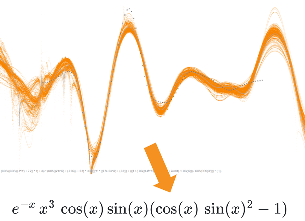
The problem? The search space is unbelievably vast and filled with redundancy.

It's all the same, no matter where you are

Imagine trying to navigate a forest with many paths leading to the same (wrong) destination, and you have to try them all until you follow one that leads you to your goal. That's the reality of Symbolic Regression. Consider the simple expression $2x$. How many different ways can you write that same value?

$$ x+x \\ \frac{4x}{2} \\ 3x-x \\ \dots \text{and many more!} $$

All these expressions are mathematically identical; they will all yield the exact same result for the same dataset.

This redundancy creates two issues for our search algorithms:

1. Wasted Time: The algorithm might revisit $x+x$ after having already explored $2x$, wasting valuable computational budget.

2. Complexity: If $x+x$ is the correct solution, we want its simplest, and most interpretable form ($2x$), not one of the infinitely complex equivalent forms. Using post-processing simplification tools often fails or introduces new problems, as we've shown in our research [1].

On the other hand, redundancy can be helpful. Sometimes, navigating from $x+x$ to $3x-x$ can be a "stepping stone" to reach a new, better area of the search space. This is known as the neutral space theory [2].

But what if we could detect all equivalent expressions in real-time and use that knowledge to make the search efficient?

A database for math expressions: the E-graph

The solution lies in E-graphs and Equality Saturation [3].

Think of an e-graph as a database for mathematical expressions. It’s designed to store many different, but equivalent, expressions with a minimum amount of space. It also makes it easier to query for expressions with certain patterns.

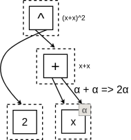
In an e-graph, symbols (such as $+, -, x, \log$) are called e-nodes. The core concept is the e-class, which acts as an equivalence group. Any e-node belonging to the same e-class represents a mathematically identical value.

For example, in the figure below, the dashed box in the middle is an e-class. It contains two e-nodes: one for multiplication (2x) and one for addition (x+x). Because they are in the same e-class, the graph automatically knows that $2x = x+x$.

This structure is immensely powerful. Now, when the graph builds a larger expression, such as a term squared (the very top multiplication operator in this e-graph), it knows it can be represented in four different ways instantly:

$$ (2x) (2x) \\ (2x) (x+x) \\ (x+x) (2x) \\ (x+x)(x+x) $$

The E-graph stores all four, but only pays the storage cost for one!

Equality saturation: automatically generating equivalence

How does the E-graph learn what's equivalent? It uses an algorithm called Equality Saturation. This process takes a simple set of mathematical rules (such as the distributive property or $a+a=2a$) and applies them repeatedly until no new equivalences can be found (or until a time limit is reached).

Let’s watch it work on the expression $(x+x)^2$ using three simple rules:

$$ \alpha + \alpha \rightarrow 2\alpha \\ \alpha \times \alpha \rightarrow \alpha^2 \\ \alpha \times (\beta + \gamma) \rightarrow (\alpha \times \beta + \alpha \times \gamma) $$

1. Start: Insert $(x+x)^2$ into the graph.

2. Apply Rules: The rule $\alpha + \alpha \rightarrow 2\alpha$ applies to the inner expression $x+x$:

3. We insert the right-hand side, $2x$, and merge it with the e-class for $x+x$, as the graph knows they are identical:

4. Repeat until Saturation: The process continues, applying other rules until the E-graph contains every possible equivalent expression derived from these rules:

The most popular implementation of equality saturation is Egg [4], a library written in Rust. But, how can e-graphs and equality saturation help with symbolic regression search?

Symbolic Regression and E-graphs, its a match 💖!

A few years ago, we realized this powerful mechanism could be the missing piece in Symbolic Regression and we pioneered their integration in different applications.

First, we demonstrated that e-graphs are a superior simplification tool compared to standard methods like sympy [1]. By simplifying equations with equality saturation, we not only reduced model complexity but also increased the probability of finding the best-fitting local optima [6].

Second, we found the E-graph structure could be used to analyze how inefficient standard search algorithms like Genetic Programming were under a limited budget, showing how often they revisited the same expressions [5] in severely length-limited and therefore constrained search spaces.

At this point, we felt there was much more we could do with e-graphs in SR.

Generating uniqueness

In our most recent work on e-graph genetic programming (eggp) [7], we turned the e-graph into a database and guidance system for equation discovery.

Remember how genetic programming works:

• Create initial random expressions
• Repeat:
  • Select two expressions proportional to their performance
  • Combine parts of these expressions generating a new expression
  • Replace a part of this expression with a random variation

As stated before, this can be inefficient since we can generate many equivalent expressions during the process [5]. But, what if we store every generated expression into a single e-graph and run the equality saturation algorithm?

For once, we would have a database system allowing us to query whether a given expression was already visited, even in an equivalent form. But also, we can use this information to enforce the generation of new expressions!

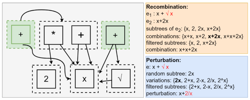
It works like this, imagine that the current state of the search is the e-graph above! The green e-classes are the root of the already evaluated expressions. Let's say that GP decides to recombine the expressions $x + \sqrt{x}$ and $x + 2x$, choosing to replace $\sqrt{x}$ of the first expression with something else from the second. The choices of recombination are ${x+x, x+2, x+2x, x+x+2x}$. We can query each one of these choices to verify whether they already exist in the e-graph. If they do and were already evaluated, we discard them!

Similarly, we can do the same for the mutation. let's suppose we will mutate the expression $x + \sqrt{x}$ by replacing $\sqrt{x}$ with a random expression. If we are unlucky, we may generate the expression $2x$, thus forming $x+2x$, which was already evaluated. After detecting the duplicate, we can change the multiplication in $2x$ with any binary operator that would generate a new expression!

Explore the Search Space with eggp and rEGGression

You can start using this algorithm right now! Here is how you can install our library and use it to find an equation for a real-world fluid dynamics dataset. You can install eggp with pip:

pip install eggp

Finding a Formula

This example uses eggp to find a relationship for one of the 'Nikuradse problems' [9] (see the tutorials at this link).

from eggp import EGGP
import pandas as pd

pd.set_option('display.max_colwidth', 100)
df = pd.read_csv("datasets/nikuradse_1.csv")

model = EGGP(gen=100, nPop=100, maxSize=15, nTournament=5, pc=0.8, pm=0.2, nonterminals='add,sub,mul,div,power,exp,log', loss='MSE', simplify=True, dumpTo='regression_example.egg')

model.fit(df[['r_k', 'log_Re']], df['target'])
print(model.results[['Expression', 'loss_train', 'loss_val', 'size']])

After running the search, the final e-graph (stored in regression_example.egg) contains the entire history of visited, unique solutions. This can be used to resume the search with different settings, such as a different nonterminal set:

model = EGGP(gen=100, nPop=100, maxSize=15, nTournament=5, pc=0.8, pm=0.2, nonterminals='add,sub,mul,div,power,exp,log,sin,tanh', loss='MSE', loadFrom='regression_example.egg')

model.fit(df[['r_k', 'log_Re']], df['target'])

print("\nLast population resumed from the first Pareto front: ")
print(model.results[['Expression', 'loss_train', 'loss_val', 'size']])

Interactive Model Selection with rEGGression

This e-graph can be further explored with the rEGGression tool [8]. An e-graph explorer for Symbolic Regression.

from reggression import Reggression

egg = Reggression(dataset="datasets/nikuradse_1.csv", loadFrom="regression_example.egg", loss="MSE")
print(egg.top(5, pattern="v0 ^ v0")

This will retrieve the top 5 expressions that follow the pattern $\alpha^\alpha$, such as $x^x$ or $\log((x+5)^{x+5}) + 3$. The result is a list of the best-performing models matching your structural criteria:

Or retrieving the top-5 expressions not having the pattern $\log(v)$:

print(egg.top(5, pattern="log(v0)", negate=True)

Conclusion

The integration of e-graphs and equality saturation is not just an academic exercise; it's a fundamental change in how we approach Symbolic Regression. By treating equivalent expressions as one, we eliminate computational waste and focus the search entirely on finding novel and better solutions.

Our eggp algorithm shows the potential of this integration, achieving state-of-the-art results with a streamlined genetic programming framework. Furthermore, rEGGression gives the human expert unparalleled power to explore the results, acting as an interactive tool for guided model selection that is agnostic to the original SR method.

The days of algorithms driving in circles are over. E-graphs have provided the GPS.

Coming up Next!

This library is not limited to just that! In the next blog post we will show how to use rEGGression to integrate and improve other algorithms!

Technical Details

Our e-graph implementation is available at the Haskell Symbolic Regression library with some differences from egg to make it more convenient for symbolic regression and memory efficient.

Our SR algorithm eggp already shows the potential of this integration, being capable of beating the state-of-the-art with a simple genetic programming framework.

The rEGGression Python library make it easy to explore the explored solutions and can be used as an interactive tool for a guided model selection.

References

[1] de Franca, Fabricio Olivetti, and Gabriel Kronberger. "Reducing overparameterization of symbolic regression models with equality saturation." Proceedings of the Genetic and Evolutionary Computation Conference. 2023.

[2] Banzhaf, Wolfgang, Ting Hu, and Gabriela Ochoa. "How the combinatorics of neutral spaces leads genetic programming to discover simple solutions." Genetic Programming Theory and Practice XX. Singapore: Springer Nature Singapore, 2024. 65-86.

[3] Tate, Ross, et al. "Equality saturation: a new approach to optimization." Proceedings of the 36th annual ACM SIGPLAN-SIGACT symposium on Principles of programming languages. 2009.

[4] Willsey, Max, et al. "Egg: Fast and extensible equality saturation." Proceedings of the ACM on Programming Languages 5.POPL (2021): 1-29.

[5] Kronberger, Gabriel, et al. "The inefficiency of genetic programming for symbolic regression." International Conference on Parallel Problem Solving from Nature. Cham: Springer Nature Switzerland, 2024.

[6] Kronberger, Gabriel, and Fabricio Olivetti de Franca. "Effects of reducing redundant parameters in parameter optimization for symbolic regression using genetic programming." Journal of Symbolic Computation 129 (2025): 102413.

[7] de França, Fabrício Olivetti, and Gabriel Kronberger. "Improving Genetic Programming for Symbolic Regression with Equality Graphs." Proceedings of the Genetic and Evolutionary Computation Conference. 2025.

[8] de França, Fabrício Olivetti, and Gabriel Kronberger. "rEGGression: an Interactive and Agnostic Tool for the Exploration of Symbolic Regression Models." Proceedings of the Genetic and Evolutionary Computation Conference. 2025.

[9] Guimerà, Roger, et al. "A Bayesian machine scientist to aid in the solution of challenging scientific problems." Science Advances Vol. 6, No. 5, eaav6971, doi: 10.1126/sciadv.aav69 2020.

The sessions for the GP track and the poster sessions had several additional contributions on SR.

It has been a while since my (Gabriel's) previous in-person visit to GECCO in 2018. For me, it was an outstanding intellectually satisfying event in Malaga, thanks to the many friends and new like-minded colleagues that I met after a long time. The many interesting and friendly chats I had in the breaks between sessions and at dinner were the best part of the conference.

Talks

Florian Bachinger presented his proposal of benchmarks for shape constrained regression which should be helpful for the development of SR algorithms that allow to incorporate knowledge on the shape of the regression function (range, monotonicity, curvature). Regression with shape constraints could for instance be helpful to restrict function behaviour outside the range of training data to improve extrapolation. The benchmark is based on an adapted version of the AI Feynman SR benchmark functions which uses physically appropriate ranges for the input variables. They derive target constraints for each benchmark instance automatically by analysing data from the known target function and its derivatives. SCR-Benchmarks

Hernan Lira presented an application of SR for identifying pathways of oceanic metabolism in the OceanIA project https://oceania.inria.cl. They use SR to describe the relationships between environmental conditions in the ocean, gene abundances and metabolism pathways in oceanic life and a large set of relevant descriptors (KO). They use several specific adaptations, such as a hierarchical (2-level) model and a multi-view approach, to find a common model structure but allow different fitting parameters for metabolism at different ocean depths. The fitness function includes several penalty terms to nudge GP to identify biologically plausible and consistent multi-view SR models. Several questions were discussed which mainly revolved around the constraints that were used to improve biological plausibility.

Fitria Wulandari presented a data augmentation idea to improve the extrapolation behavior of SR models. The approach is based on generating synthetic data outside of the region of training data (extrapolation range) from a teacher model. The teacher model is trained only on the available data but allows to freely generate additional training data for SR. The hypothesis is that the bias of the teacher model can lead to useful synthetic data (probably: lower noise, smooth) for SR. Different algorithms were tried for the teacher model (NN, RF, GBT, SR) and the performance of SR with and without teacher model was compared. Results seem to be mixed / inconclusive.

Alberto Tonda showed an example where data transformation can mislead search. This problem appears for example in symbolic system identification, that is finding ordinary differential equations that predict the dynamics of systems based solely on samples of observed states from the system. Alberto showed that two options for solving this problem both involve data transformation. Here this refers to adding calculated columns for the approximated derivatives of trajectories to the dataset that are used as the target for symbolic regression. By this the symbolic identification problem is converted to a symbolic regression problem which is beneficial as it is easier to evaluate a loss function (no numeric integration) but on the other hand requires smoothing of the approximate derivatives. They used Savitzky-Golay smoothing and tuned hyperparameters for the smoother. The result was tested on ODEBench whereby for some instances the data transformation led to a misleading fitness function (the loss of the true data generating function was higher than the loss of the identified function). Discussion revolved around the characteristics around the problematic instances (more wiggly or more chaotic?).

Jiajun Duan presented results using a well-known benchmark dataset from the medical domain (Parkinson’s) to argue that using a hinge-loss function for the classification problem instead of accuracy is beneficial but admits that the hinge loss does not match typical likelihood functions for classification problems.

Bernhard Werth revisited pruning in tree-based GP for SR. Pruning is the removal of ineffective subexpressions with the motivation to make space for beneficial growth of expressions, ideally reducing size and/or improving prediction error. The looked at continuous pruning which means pruning a part or all of the trees in each generation, not just at the end. The empirical results on a large set of datasets did show an improvement in training and test quality but did not show a clear difference in model length between GP with and without pruning. One explanation given by the speaker was that strict offspring selection (a specific variant of GP developed in the group) immediately fills up the pruned subexpressions with other expressions of similar size.

Erik-Jan Senn presented his preliminary work on establishing theoretical statements about the limit-behaviour model selection consistency and efficiency of symbolic regression algorithms. The main motivation being to see whether SR algorithms can identify the “true model” or the best approximation in the limit of infinite number of observations. He introduced an abstract formulation of all SR algorithms as two-phase model selection approaches and conjectures that exhaustive symbolic regression (Bartlett et al.) selects the correct functional form in large samples (with the assumption that the parameter fitting problem is solved by an oracle). He did not make a similar statement about GP yet but argues that the PAC framework should be revisited to get a better understanding about the theoretical guarantees of SR. How this affects practical applications was not covered.

Guilherme Imai Almeida presented the recent modifications of SRBench and new results. To reduce runtime for running all the experiments the number of datasets was reduced by selecting the datasets that were most discriminative among the different algorithms via a dimensionality reduction and agglomerative clustering. The dataset features for this clustering were descriptive features such as the size (number of observations and variables), best R², as well as performance results of algorithms. A focus of recent SRBench work was to allow more detailed comparisons between algorithms on individual datasets instead of aggregating all results into a single rank for comparison (benchmarking is not about finding a winner but instead should give us insights in the relative weaknesses and open issues of existing implementations). In the discussion the point was raised that it is still useful to have the simple ranking of algorithms because outsiders are mainly interested in finding out what is the “best” method on average that can be used.

Nathan Haut presented result of using alternating tournaments in GP with three objectives, prediction error, expression complexity (visitation length), and smoothness of the regression function. They used alternating Pareto tournaments in two objectives, that is, if in one generation they select the Pareto optimal individuals regarding prediction error and complexity they would switch this to prediction error and smoothness in the next generation. Many different variations for alternating Pareto tournaments were evaluated on the Kotanchek test function and several other benchmark datasets and positive results were observed: prediction errors, complexity and smoothness could be improved on average. As a remark about the motivation for using Pareto tournaments instead of doing multi.-objective NSGA-II directly, Nathan mentioned that Pareto tournaments in his experience focus more on the most important region/knee of the Pareto front instead of keeping the whole Pareto front in the population.

Discussion

After the talks we have a lively 30-minute long discussion round allowing all participants to express their thoughts about the most pressing topics in SR research.

Stability

An issue raised was stability of GP for SR. While there is some degree of semantic stability which leads to comparable prediction errors of the produced models from multiple GP runs, the expressions can be completely different each time. This is problematic in scientific and engineering applications because it reduces trust in in the results and requires more effort in the validation or interpretation of the expressions to gain knowledge about the studied systems. Stability is a beneficial property for SR algorithms and it is worthwhile to improve current systems in this direction. Recent work on using equality saturation and egraphs, also presented in other tracks at GECCO could help here.

Uncertainty

The next topic was handling uncertainty of SR models. We are frequently just assuming exact data points (discarding data / measurement uncertainty) and often use a loss function such as negative R² or sum of squared errors to assess model fit. First, we should start including an error model for the data; uncertainty of data propagates into uncertainty of parameters, and further into uncertainty of predictions giving e.g. confidence intervals for parameters or prediction intervals. Including this uncertainty has other benefits in model selection, overfitting reduction, and preventing unnecessarily complexity models. Beyond that the model selection uncertainty through GP search is another factor. On the other hand, there can be difficulties expression confidence regions or prediction intervals when combining multiple models into an ensemble or with multi-modal likelihood functions (not sure if I understood the online comment correctly). In any case, recent work in Bayesian symbolic regression and sequential Monte Carlo sampling for symbolic regression looks very promising.

Benchmarks

Several participants raised the question: “What benchmarks should we use or what are characteristics of good benchmark problems?”. There seems to be a consensus that most of the AI Feynman problem instances are too easy as they are very short expressions that can be recovered easily with exhaustive search. We should question whether it is worthwhile to devise intricate SR systems to be able to discover such simple equations. Probably we should construct much more complex synthetic benchmark functions to really challenge our current SR systems. On the other hand, if such complex target functions never occur in real-world situations directing efforts into systems that are able to rediscover such equations might also be wasted. We should not dump all problem instances (and algorithms) into the same bin but instead could use groups of characteristically similar instances.

More

We discussed the aims of SR implementations. Currently, SR is often considered as a solver or a system giving you a solution for a problem, instead SR could be more useful as an exploration tool (such as rEGGression which was presented in another GECCO track). Both use cases are beneficial.

Another topic was the smoothness of mutation in genetic programming. Typical mutation operators are rather disruptive, and the hypothesis was raised that a smoother mutation operation could improve search.

Gabriel Kronberger and Fabrício Olivetti de Franca

Symbolic regression is a branch of machine learning that attempts to find interpretable mathematical expressions which can accurately approximate a data set. This meeting brought together practitioners of symbolic regression with physicists who are tackling problems which are particularly amenable to their analysis.

Left to right: C. Cornelio, E. Kabliman, S. Manti, A. Lucantonio, L. Kammerer, G. Kronberger, H. Desmond, A. Soltani, D. Bartlett, G. Bomarito, N. Kutz, F. Olivetti de Franca, P. Ferreira, B. Burlacu, W. La Cava, A. Constantin

Schedule

The workshop had a mixture of talks focussing either on applications of symbolic regression in physical sciences and engineering or on symbolic regression methods.

Monday 28th of April:

• Harry Desmond, University of Portsmouth, (Exhaustive) Symbolic Regression and model selection by minimum description length Video
• Steven Abel, Durham University, Symbolic regression in beyond Standard Model physics Video
• Evgeniya Kabliman, University of Bremen & Leibniz Institute for Materials Engineering, Constitutive modelling using symbolic regression Video
• Roger Guimerà, Universitat Rovira i Virgili Physics for symbolic regression, Symbolic regression for physics Video
• William La Cava, Boston Children's Hospital Brush: incorporating split-wise functions and multi-armed bandits into symbolic regression Video
• Tariq Yasin, University of Oxford, Empirical dark matter profiles with symbolic regression Video
• Cristina Cornelio, Samsung AI, Derivable scientific discovery Video
• J. Nathan Kutz, University of Washington, Sparse regression for symbolic representations in latent space dynamics Video

Tuesday 29th of April:

• Deaglan Bartlett, Institut d'Astrophysique de Paris, Accelerating cosmological modelling with symbolic regression Video

• Miles Cranmer, University of Cambridge, Concept evolution and SymbolicRegression.jl as a modular research platform Video

• Etienne Russeil, Stockholm University, Multi-view Symbolic Regression: from independent experiments to general laws Video

• Geoffrey Bomarito, National Aeronautics and Space Administration (NASA), Symbolic regression via posterior sampling Video

• Andrei Constantin, University of Birmingham & University of Oxford, Statistical patterns in the equations of physics and the emergence of a meta-law of Nature Video

• Bogdan Burlacu, University of Applied Sciences Upper Austria, Zobrist hash-based duplicate detection in symbolic regression Video

• Fabricio Olivetti de França, Universidade Federal do ABC, Equality graph assisted symbolic regression Video

• Panel Discussion and Closing

Summary

Several speakers gave excellent examples showcasing the power of symbolic regression and its ability to produce fast and accurate models. Several issues and ideas were raised repeatedly by different speakers. These recurring themes include additional quality criteria for SR models for instance to preferably produce physically plausible and interpretable models, hierarchical models with global parameters and local fitting parameters for each dataset, and systematic handling of data and model uncertainty.

Additional quality criteria

Measurements of accuracy, such as the mean of squared errors, capture how well a certain model fits data but cannot always tell if such models are going to be useful when put into practice. Because of that, a recurrent topic in the workshop was the use of additional quality criteria for candidate expressions.

For example, in Exhaustive Symbolic Regression as explained by Harry Desmond, minimizing the description length can bias the search toward a balance between accuracy and complexity while taking the uncertainty of the data into consideration. The minimum description length principle is connected to maximizing Bayesian evidence under different model priors. Using what they called the Katz prior they tried to produce expressions with a similar distribution of operators as exhibited by a list of named equations collected from Wikipedia.

The talk of Roger Guimerà about the Bayesian Machine Scientist was similar in idea. He discussed a prior for the structure of the function based on the already established physics equation to ensure that the accumulated knowledge throughout history is taken into consideration for biasing the search of expressions.

If we have prior knowledge about logical constraints and axioms which the final model must follow, it is possible to select hypotheses that conform to such constraints or to create a feedback for the search engine to sample new candidates. Cristina Cornelio argued that this guidance helps to find correct models in their systems called AI Descartes and AI Hilbert.

There was a lively discussion about the ability of SR to discover physical equations, which often exhibit certain specific characteristics (the formula looks "physical"). Andrei Constantin presented his thoughts on a meta-law of Nature circling around peculiar statistical patterns that occur in the equations of physics.

The aim to find interpretable models is closely connected with the idea of using priors to produce natural or physical expressions. William La Cava showed some examples in the medical domain, where he used an implementation of symbolic regression and genetic programming called Brush to produce interpretable models similar to decision trees that help physicians and patients understand the reasoning for diagnoses. Additionally, he argued for the need for a benchmark or competition that evaluates interpretability of symbolic regression results. Discussion revolved around the problem of defining and measuring interpretability.

Sampling from the posterior distribution of expressions can lead to a Bayesian view of how to handle uncertainties. Geoffrey Bomarito showed how this can be exploited to gradually introduce the effect of data into the search promoting an improved capability of retrieving the true expression under limited, noisy, and sparse data.

Steven Abel used symbolic regression tools in the context of finding extensions to the Standard Model of particle physics by trying to find accurate and efficient emulators for computationally heavy numerical simulations. He presented a huge expression produced by PyOperon spanning a whole slide. To produce an expression that is accurate for inputs which are most relevant for the numerical simulation they used a simple weighting scheme with PyOperon to weight those data more heavily.

The execution speed of the symbolic regression models is another relevant quality criterion, for example when using SR models in the form of emulators in larger optimization pipelines. This was raised for instance by Deaglan Bartlett when he presented his results for finding emulators for the linear and non-linear power spectrum of pairwise galaxy distances and again when he presented the beautiful new approximation for a hypergeometric function that was more accurate than the human-derived approximation which has been used for decades. In this talk on SymbolicRegression.jl and PySR, Miles Cranmer expressed that he thinks that probably the best criterion for model complexity is the speed of evaluating the expressions on an FPGA.

Overall, with that many possibilities of calculating the quality of the obtained solutions, there is a need for a customizable experience with symbolic regression tools. Miles Cranmer showed his recent improvements with PySR and how it is capable of incorporating customized loss functions, operators, and function templates in the form of standard Julia code even allowing the importing of external libraries (such as ODE solvers). As some decisions can be made post-hoc, there may be a need for a structured database of hypothesis that can be easily explored by the user; this can be accomplished with the equality graphs, presented by Fabricio Olivetti de França, allowing the automatic derivation of properties (i.e., monotonicity), pattern matching, and statistics on common patterns observed during the search.

Hierarchical models

In most of the talks, symbolic regression models were used as one component embedded within a larger pipeline or hierarchical simulation model. Different ways of handling this were mentioned in several talks.

For example Roger Guimerà showed ordinary differential equations produced by the Bayesian Machine Scientist which describe the growth behaviour of bacterial strains on different media. The system found a common expression which was accurate for all growth curves but had fitting parameters that were fit to each of the individual growth curves. Similarly, the expressions found by the Bayesian Machine Scientists for predicting mobility patterns between larger cities included fitting parameters tuned for each city. Etienne Russeil called this approach multi-view symbolic regression and he highlighted results for example for the observed light intensity curves of supernovae over time where symbolic regression was used to find a common model structure with parameters that are fit to each supernova light curve.

Tariq Yasin also mentioned a similar approach with global parameters and local parameters fit to each of the approximately 150 galaxies in the dataset that they used.

Evgeniya Kabliman presented the idea to use symbolic regression to find short expressions that can be used to calculate the local parameters from other known variables instead of fitting the parameters to each dataset. Her work is focused on the development of constitutive models explaining mechanical properties of metallic materials. In this domain, several physics-based models exist to describe stress-strain behaviour but all models still have fitting parameters that must be estimated from costly measurements. She proposed using SR to improve such physics-based models by finding expressions which allow to replace fitting parameters. A main issue in these models seems to be that uncertainty of measurements and variability of samples used in experiments is often ignored.

Nathan Kutz presented an approach called Sensing with shallow recurrent decoder networks (SHRED) and it combination with sparse identification of nonlinear dynamics (SINDy) to produce sparse spatio-dynamical models. SHRED uses a recurrent neural network architecture (LSTM) with a final decoder layer to learn and predict noisy dynamical processes. The data is compressed into a latent space which makes it easier to produce accurate and robust predictions. He also repeatedly mentioned the unexpected difficulty of numerically approximating derivatives of noisy functions.

Systematic handling of data and model uncertainty

One potential shortcoming of current SR research, highlighted in the workshop, is the insufficient consideration given to the issue of uncertainty quantification. Looking at the data and models in terms of likelihoods provides a principled way for dealing with overfitting and selecting generalizable models. Unfortunately, this aspect is often ignored and hardly discussed in current symbolic regression work. During the workshop, the main presented approaches to handle uncertainty was the minimization of description length, presented in Harry's talk and the Bayesian approach by Geoffrey that incrementally take the data uncertainty into consideration.

Efficiency and usability of SR tools

As SR becomes more popular, it is necessary to ensure a good experience for the final user. This points to efficiency, ease of use, and customization. Regarding efficiency, PyOperon already provides an optimized implementation often orders of magnitude faster than other approaches. Bogdan Burlacu showed that it is still possible to improve the runtime by caching the fitness values for already visited expressions using the Zobrist hash. With this approach, he avoided evaluating repeated expressions along the search. Similar to this idea, Fabricio Olivetti also exploited the fact that equality graphs can represent equivalence relationships, thus stimulating the generation of unique expressions and improving the speed of convergence. He also argued that many implementations contain too many hyper-parameters, which are not often intuitive to the user, and he showed that a minimum set of hyper-parameters can be enough to achieve competing results with the popular implementations. Finally, regarding customization, as already mentioned, Miles Cranmer introduced many new features to PySR enabling the user to adapt the main components to fit their personal demands. A briefly presented alternative was r🥚ression (aka rEGGression) that exploits equality graphs to offer a post-analysis navigation of multiple models found by a combination of SR algorithm executions.

Operon and PyOperon

Operon seems to be a popular framework for astrophysics. It has been used in many works presented at the workshop.

Application examples

• Deaglan Bartlett et al. used PyOperon to develop a symbolic emulator for the linear matter power spectrum
  • https://github.com/DeaglanBartlett/symbolic_pofk
  • https://arxiv.org/abs/2311.15865
• Steve Abel et al. used Operon to develop analytical expressions for beyond Standard Model physics
• Etienne Russeil et al. used PyOperon for Multi-View Symbolic Regression with applications to phenomenological modeling https://arxiv.org/abs/2405.18471
• Evgeniya Kabliman et al. used PyOperon for modeling stress-strain curves of aluminium and steel alloys

Feature requests

In general, it would seem that the current scikit-learn interface provided by pyoperon is not very flexible and more attention should be paid to ergonomics, ease-of-use and customization.

Summary of requested features:

• support for a wider range of likelihoods, and the possibility to fully specify the data uncertainties in the form of a covariance matrix
• support for custom loss functions (note: this is already possible with the UserDefinedEvaluator, but it poses some issues in the Python wrapper due to the GIL/concurrency issues)
• support for constraining the number of model parameters
• the ability to perform restarts during parameter tuning
• support for warm starts and, more generally, seeding the initialization or resuming the search with an existing population

Future Activities

• Symbolic Regression Workshop at the Genetic and Evolutionary Computation Conference (GECCO) 14th-18th of July, Malaga
• Advancing Computational Mechanics with Symbolic Regression, U.S. National Congress on Computational Mechanics, Chicago July 20-24, 2025
• We plan to organize a workshop proposal at NeurIPS in December 2025

We had a great time in London and enjoyed the insightful talks. We thank the Royal Society for hosting and funding this meeting.